Autoencoders

An autoencoder [Bengio09] is a network whose graphical structure is shown in Figure 4.1, which has the same dimension for both input and output. It takes an unlabeled training examples in set where is a single input and encodes it to the hidden layer by linear combination with weight matrix 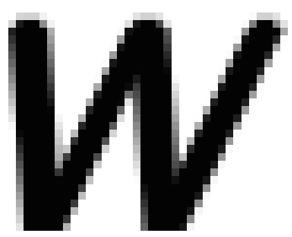and then through a non-linear activation function. It can be mathematically expressed as , where 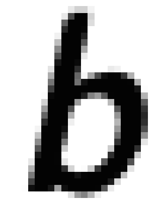is the bias vector.

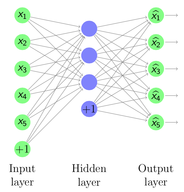
Figure 4.1: An Autoencoder

After that the hidden layer representation will be reconstructed to the output layer 􏰌 through a decoding function, in which 􏰌 has a same shape as . Hence the decoding function can be mathematically expressed as 􏰌, where can be called tried weights. In this project, tied weights were used. The aim of the model is to optimize the weight matrices, so that the reconstruction error between input and output can be minimized. It can be seen that the Autoencoder can be viewed as an unsupervised learning process of encoding-decoding: the encoder encodes the input through multi-layer encoder and then the decoder will decode it back with the lowest error [Hinton06].
To measure the reconstruction error, traditional squared error can be used. One of the most widely used way to measure that is the cross entropy if the input can be represented as bit vector or bit possibilities. The cross entropy error is shown in Equation 4.1:

Equation:4.1

The hidden layer code can capture the information of input examples along the main dimensions of variant coordinates via minimizing the reconstruction error. It is similar to the principle component analysis (PCA) which project data on the main component that captures the main information of the data. h can be viewed as a compression of input data with some lost, which hopefully not contain much information about the data. It is optimized to compress well the training data and have a small reconstruction error for the test data, but not for the data randomly chosen from input space.

Denoising Autoencoders

In order to prevent the Autoencoder from just learning the identity of the input and make the learnt representation more robust, it is better to reconstruct a corrupted version of the input. The Autoencoder with a corrupted version of input is called a Denoising Autoencoder. Its structure is shown in Figure 4.2. This method was proposed in [Vincent08], and it showed an advantage of corrupting the input by comparative experiments. Hence we will use denoising autoencoders instead of classic autoencoders in this thesis.

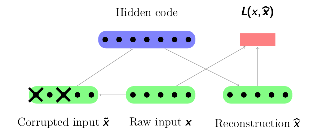
Figure 4.2: A graphical figure of Denoising Autoencoder. An input x is corrupted to . After that the autoencoder maps it to the hidden representation and attempts to reconstruct .

A Denoising Autoencoder can be seen as a stochastic version with adding a stochastic corruption process to Autoencoder. For the raw inputs , some of them will be randomly set to 0 as corrupted inputs . Next the corrupted input will be en- coded to the hidden code and then reconstructed to the ouput. But now 􏰌 is a deterministic function of rather than . As Autoencoder, the reconstruction is considered and calculated between 􏰌 and noted as . The parameters of the model are initialized randomly and then optimized by stochastic gradient descent algorithms. The difference is that the input of the encoding process is a corrupted version , hence it forces a much more clever mapping than just the identity, which can denoise and extract useful features in a noise condition.

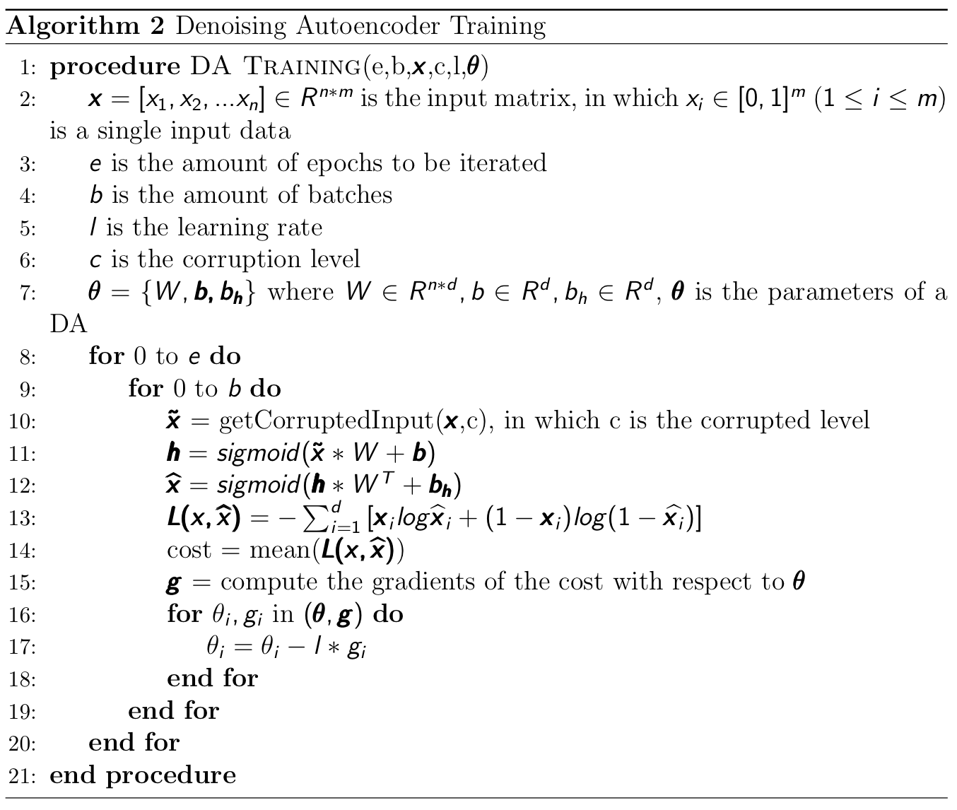
The training algorithm of a denoising autoencoder is summarized in Algorithm 2.

Stacked Autoencoder

Unsupervised pre-training
A Stacked Autoencoder is a multi-layer neural network which consists of Autoencoders in each layer. Each layer’s input is from previous layer’s output. The greedy layer wise pre-training is an unsupervised approach that trains only one layer each time. Every layer is trained as a denoising autoencoder via minimising the cross entropy in reconstruction. Once the first layer has been trained, it can train the layer by using the previous layer’s hidden representation as input. An example is shown below. Figure 4.3 shows the first step of a stacked autoencoder. It trains an autoencoder on raw input to learn by minimizing the reconstruction error .

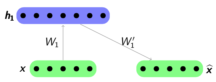
Figure 4.3: Step 1 in Stacked Autoencoders

Next step shown in Figure 4.4. The hidden representation would be as ”raw input” to train another autoencoder by minimizing the reconstruction error . Note that the error is calculated between previous latent feature representation and the output . Parameters and will be optimized by the gradient descent algorithm. The new hidden representation h2 will be the ’raw input’ of the next layer.

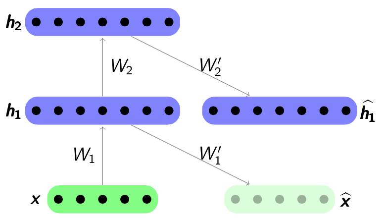
Figure 4.4: Step 2 in Stacked Autoencoders

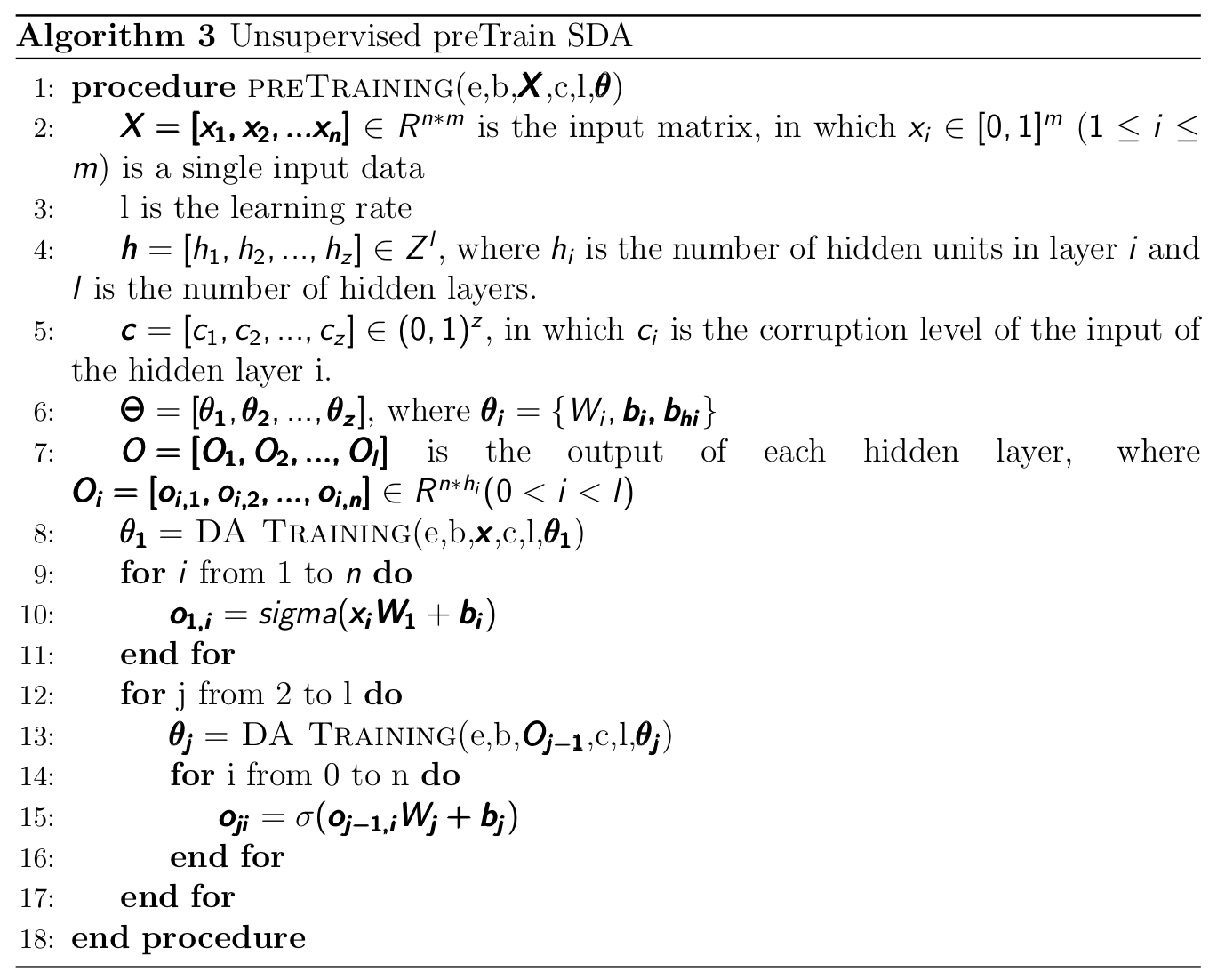
The pre-training algorithm of stacked denoising autoencoder is summarized in algorithm 3.

Supervised fine-tuning

At last once all the layers has been pre-trained, the next step called fine-tuning is performed. A supervised predictor will be extended to the last layer, such as support vector machine or a logistic regression layer. In this project, we chose a logistic regression layer. After that the network will be trained. A sample graph is shown in Figure 4.5. It can be seen that for each layer of the network, only the encoding hidden representation are considered. The fine-tuning step will train the whole network by back-propagation like training an Artificial Neural Network. A stacked denoising autoencoder is just replace each layer’s autoencoder with denoising autoencoder whilst keeping other things the same.

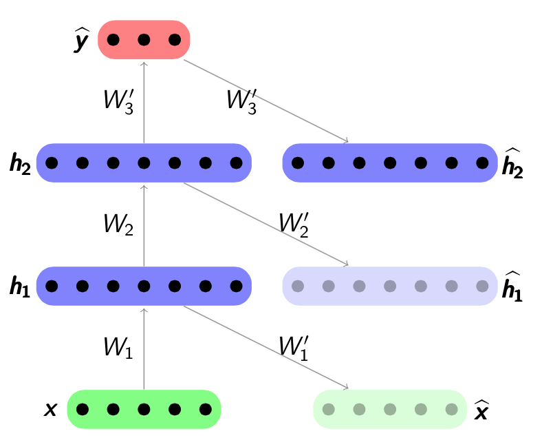
Figure 4.5: A complete architecture of stacked autoencoder

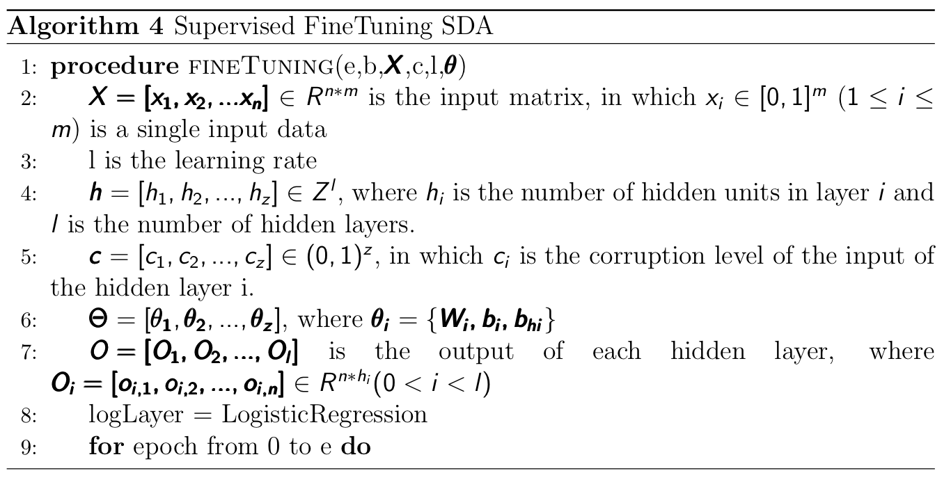
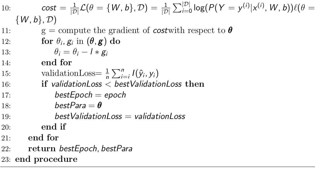
The supervised fine-tuning algorithm of stacked denoising auto-encoder is summa- rized in Algorithm 4.

[Bengio09] Yoshua Bengio. Learning deep architectures for AI. Foundations and Trends in Machine Learning, 2(1):1–127, 2009. Also published as a book. Now Publishers, 2009.

[Hinton06] Geoffrey E Hinton and Ruslan R Salakhutdinov. Reducing the dimensionality of data with neural networks. Science, 313(5786):504–507, 2006

[Vincent08] Pascal Vincent, Hugo Larochelle, Yoshua Bengio, and Pierre-Antoine Man- zagol. Extracting and composing robust features with denoising autoencoders. In Proceedings of the 25th international conference on Machine learning, pages 1096–1103. ACM, 2008.