Sentiment Classification on Large Movie Reviews
Sentiment Analysis is understood as a classic natural language processing problem. In this example, a large moview review dataset was chosen from IMDB to do a sentiment classification task with some deep learning approaches. The labeled data set consists of 50,000 IMDB movie reviews (good or bad), in which 25000 highly polar movie reviews for training, and 25,000 for testing. The dataset is originally collected by Stanford researchers and was used in a 2011 paper, and the highest accuray of 88.33% was achieved without using the unbalanced data. This example illustrates some deep learning approaches to do the sentiment classification with BigDL python API.
Load the IMDB Dataset
The IMDB dataset need to be loaded into BigDL, note that the dataset has been pre-processed, and each review was encoded as a sequence of integers. Each integer represents the index of the overall frequency of dataset, for instance, ‘5’ means the 5-th most frequent words occured in the data. It is very convinient to filter the words by some conditions, for example, to filter only the top 5,000 most common word and/or eliminate the top 30 most common words. Let’s define functions to load the pre-processed data.
1 | from dataset import base |
Processing text dataset
finished processing text
In order to set a proper max sequence length, we need to go througth the property of the data and see the length distribution of each sentence in the dataset. A box and whisker plot is shown below for reviewing the length distribution in words.
1 | # Summarize review length |
Review length:
Mean 233.76 words (172.911495)
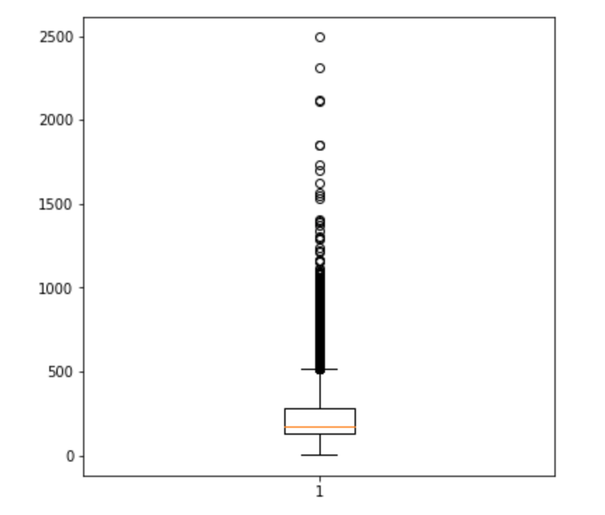
Looking the box and whisker plot, the max length of a sample in words is 500, and the mean and median are below 250. According to the plot, we can probably cover the mass of the distribution with a clipped length of 400 to 500. Here we set the max sequence length of each sample as 500.
The corresponding vocabulary sorted by frequency is also required, for further embedding the words with pre-trained vectors. The downloaded vocabulary is in {word: index}, where each word as a key and the index as a value. It needs to be transformed into {index: word} format.
Let’s define a function to obtain the vocabulary.
1 | import json |
Processing vocabulary
finished processing vocabulary
Text pre-processing
Before we train the network, some pre-processing steps need to be applied to the dataset.
Next let’s go through the mechanisms that used to be applied to the data.
We insert a
start_charat the beginning of each sentence to mark the start point. We set it as2here, and each other word index will plus a constantindex_fromto differentiate some ‘helper index’ (eg.start_char,oov_char, etc.).A
max_wordsvariable is defined as the maximum index number (the least frequent word) included in the sequence. If the word index number is larger thanmax_words, it will be replaced by a out-of-vocabulary numberoov_char, which is3here.Each word index sequence is restricted to the same length. We used left-padding here, which means the right (end) of the sequence will be keep as many as possible and drop the left (head) of the sequence if its length is more than pre-defined
sequence_len, or padding the left (head) of the sequence withpadding_value.
1 | def replace_oov(x, oov_char, max_words): |
start transformation
finish transformation
Word Embedding
Word embedding is a recent breakthrough in natural language field. The key idea is to encode words and phrases into distributed representations in the format of word vectors, which means each word is represented as a vector. There are two widely used word vector training alogirhms, one is published by Google called word to vector, the other is published by Standford called Glove. In this example, pre-trained glove is loaded into a lookup table and will be fine-tuned during the training process. BigDL provides a method to download and load glove in news20 package.
1 | from dataset import news20 |
loading glove
finish loading glove
For each word whose index less than the max_word should try to match its embedding and store in an array.
With regard to those words which can not be found in glove, we randomly sample it from a [-0.05, 0.05] uniform distribution.
BigDL usually use a LookupTable layer to do word embedding, so the matrix will be loaded to the LookupTable by seting the weight.
1 | print('processing glove') |
processing glove
finish processing glove
Build models
Next, let’s build some deep learning models for the sentiment classification.
As an example, several deep learning models are illustrated for tutorial, comparison and demonstration.
LSTM, GRU, Bi-LSTM, CNN and CNN + LSTM models are implemented as options. To decide which model to use, just assign model_type the corresponding string.
1 | from nn.layer import * |
Optimization
Optimizer need to be created to optimise the model.
Here we use the CNN model.
More details about optimizer in BigDL, please refer to Programming Guide.
1 | from optim.optimizer import * |
creating: createSequential
creating: createLookupTable
creating: createRecurrent
creating: createGRU
creating: createSelect
creating: createLinear
creating: createDropout
creating: createReLU
creating: createLinear
creating: createSigmoid
creating: createBCECriterion
creating: createMaxEpoch
creating: createAdam
creating: createOptimizer
creating: createEveryEpoch
To make the training process be visualized by TensorBoard, training summaries should be saved as a format of logs.
With regard to the usage of TensorBoard in BigDL, please refer to BigDL Wiki.
1 | import datetime as dt |
creating: createTrainSummary
creating: createSeveralIteration
creating: createValidationSummary


<optim.optimizer.Optimizer at 0x7fa651314ad0>
Now, let’s start training!
1 | %%time |
Optimization Done.
CPU times: user 196 ms, sys: 24 ms, total: 220 ms
Wall time: 51min 52s
Test
Validation accuracy is shown in the training log, here let’s get the accuracy on validation set by hand.
Predict the test_rdd (validation set data), and obtain the predicted label and ground truth label in the list.
1 | predictions = train_model.predict(test_rdd) |
Then let’s see the prediction accuracy on validation set.
1 | correct = 0 |
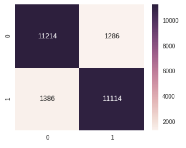
Prediction accuracy on validation set is: 0.89312
Show the confusion matrix
1 | %matplotlib inline |
<matplotlib.axes._subplots.AxesSubplot at 0x7fa643fe0c50>
Because of the limitation of ariticle length, not all the results of optional models can be shown respectively. Please try other provided optional models to see the results. If you are interested in optimizing the results, try different training parameters which may make inpacts on the result, such as the max sequence length, batch size, training epochs, preprocessing schemes, optimization methods and so on. Among the models, CNN training would be much quicker. Note that the LSTM and it variants (eg. GRU) are difficult to train, even a unsuitable batch size may cause the model not converge. In addition it is prone to overfitting, please try different dropout threshold and/or add regularizers (abouth how to add regularizers in BigDL please see BigDL Wiki).
Summary
In this example, you learned how to use BigDL to develop deep learning models for sentiment analysis including:
- How to load and review the IMDB dataset
- How to do word embedding with Glove
- How to build a CNN model for NLP with BigDL
- How to build a LSTM model for NLP with BigDL
- How to build a GRU model for NLP with BigDL
- How to build a Bi-LSTM model for NLP with BigDL
- How to build a CNN-LSTM model for NLP with BigDL
- How to train deep learning models with BigDL
Thanks for your reading, please enjoy the trip on using BigDL to build deep learning models.